When I first saw Ben Fry’s All Streets, I thought, “WOW, I need to learn how to make that!” And, a few years later Nathan Yau created a nice tutorial explaining how one could do so in R1. On a recent Thursday night, I felt lethargic from the recent Daylight Savings “Spring Forward” and the chill outside. Focus came to me slowly, though, and I decided I wanted to make a map for my home area: Durham.
Since you probably can’t see Nathan’s great tutorial, I’ll give you the gist: take US Census shapefile data, import into R with the maptools package, and use R’s built-in graphics functions to draw a map.
Finding data turned out to be somewhat of a hassle. The US Census FTP site kept timing out. I guess after work hours, there’s no guarantee. Fortunately, their website frontend was slightly more reliable (for some of these files, frustratingly, I ended up coming back the next day). The real trick to downloading data is figuring out what data to download!
A consultation of the State FIPS
codes, revealed
North Carolina to be magical number 37. Consulting the NC FIPS Codes
reference,
revealed Durham County to be magical number 063. Thusly equipped with the
magical combination 37063, I could deduce that the proper
Shapefile of roads for Durham County,
NC is tl_2016_37063_roads.zip.
With just a smidgeon of R, I got started:
library(maptools)
quartz()

roads <- readShapeLines('./tl_2016_37063_roads.shp')
par(mar=c(0,0,0,0))
plot(roads)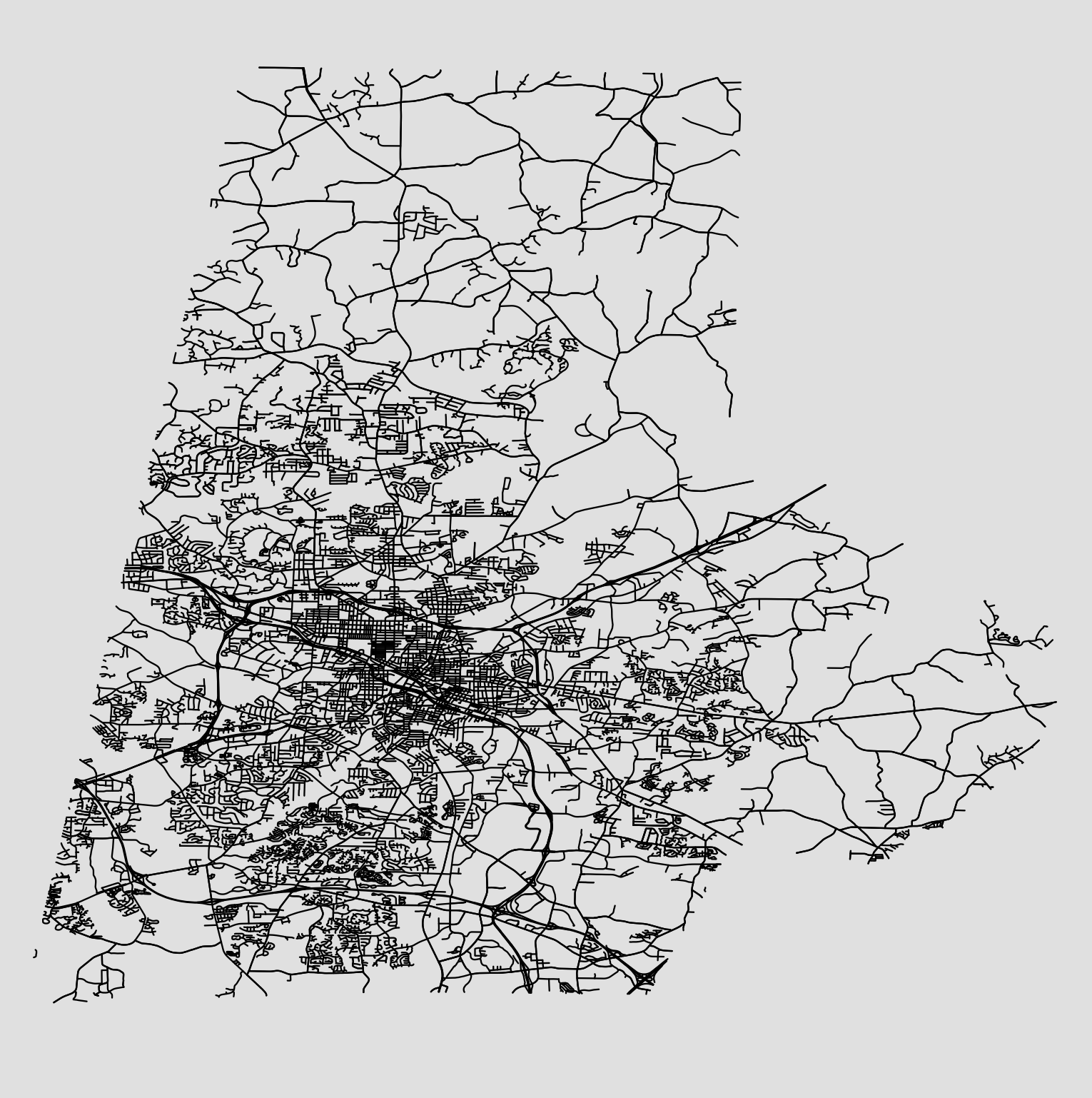
Nathan’s post focused mostly on how one might style and combine data to end up with state and national maps. Fortunately, since I am more interested in county level, I don’t have to worry about combining Shapefile data. But I wanted to include the county’s shape as an outline, I thought. I also wanted to make Interstate and State roads more prominent than a neighborhood street.
I found the county
shapes
on the same website. To figure out what sort of road each line was, I had to
decipher the roads dataframe:
> summary(roads$RTTYP)
   I    M    O    S    U NA's
   7 6034   15  430   47  514
The roads zip file came with an XML file tl_2016_37063_roads.shp.xml, which
serves as a data dictionary for the Shapefile. I is Interstate, S is State
Road, etcetera. Armed with this little knowledge I could bring a little style to
my map by varying the line width lwd and coloring the lines:
library(maptools)
quartz()

roads <- readShapeLines('./tl_2016_37063_roads.shp')
counties <- readShapePoly('./tl_2016_us_county.shp')
durham <- subset(counties, STATEFP == 37 & COUNTYFP == '063')

par(mar=c(0,0,0,0), bg='#e0e0e0')
plot(durham, col='#ffffff', border=F)
# Interstate and Highways:
lines(subset(roads, RTTYP == "U"), col="#737373", lwd=1)
lines(subset(roads, RTTYP == "I"), col="#737373", lwd=1)
# State roads:
lines(subset(roads, RTTYP == "S"), col="#737373", lwd=0.8)
# Everything else:
lines(subset(roads, !(RTTYP %in% c('S','U','I'))), col="#737373", lwd=0.5)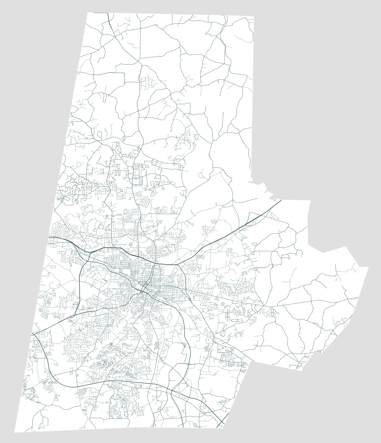
I felt pretty good. I stepped back to admire my map and wondered what all the little gaps are. Why aren’t there roads in the South West? And, hey, it kinda looks weird not having Falls Lake in the East. I decided to add water to my maps.
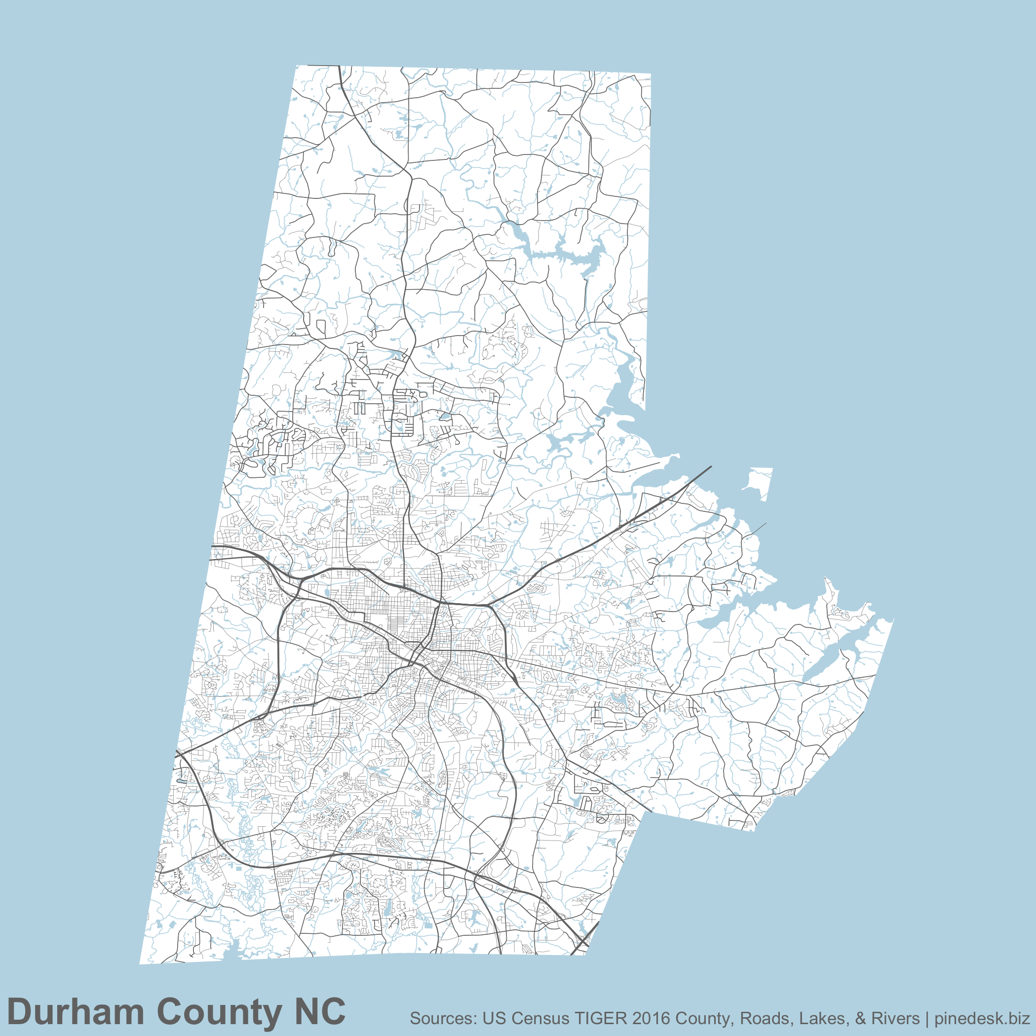
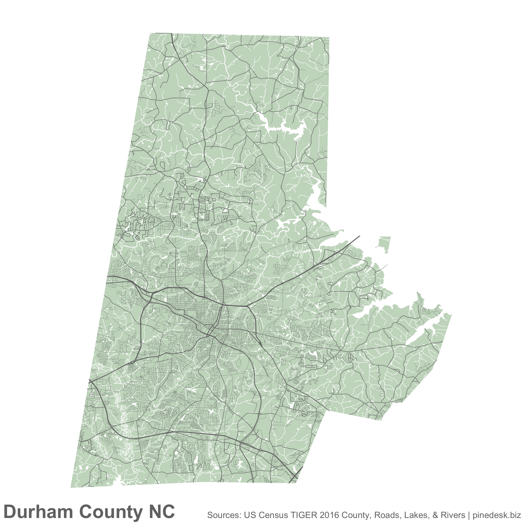
Adding multiple polygon data sets to the map tripped me up a little bit, but in all my final effort was not overly complicated: add more Shapefiles for waterways, and water areas, and add legends. Here is the final script
Stylistically I wanted to keep with the aesthetic of All Streets and create a map with a minimal number of colors, and minimal number of explanatory graphing (like, the county border). Let the data speak for itself. I couldn’t decide whether to let the ground be white, or the water be white. So, here are both:
1 Sorry, members only! If you are interested in making beautiful visualizations in R, I highly recommend obtaining a membership.